Chapter 4 Introduction to Spreadsheets
Contents
Chapter 4 Introduction to Spreadsheets
Absolute
and Relative Cell Addresses
What’s
Wrong with these functions /spreadsheets
Spreadsheet Basics
|
Spreadsheet Basics 1.
Always give a Label to your numbers so that you
know what the number stands for. 2.
Always use a Cell Reference when possible, and use
Absolute and Relative cell references as needed. 3.
Avoid having Blank Columns, set your column width instead. 4.
Verify
all your formulas and functions by hand first to be sure it produces the
correct result. Figure 1 |
With a word processor you manipulate words in your document. In a spreadsheet you use the computer to manipulate numbers. Spreadsheets are predominately used for number crunching. Spreadsheets make an excellent tool to create a budget, financial forecast, and basically anything that deals with columns, numbers and formulas. Please pay attention to the spreadsheet basics in Figure 1 as they will help you do things the right way the first time. Don’t forget the computer basics from chapter 3 as they relevant forever!
Spreadsheets have been used for years, manually, long before the computer was invented. Accountants used a spreadsheet or worksheet to prepare their budgets and other tasks. The accountants would use a pencil and paper with columns and rows. They would place the accounts in one column, the corresponding amount in the next column, etc. Then they would manually total the columns and rows. This works fine, except when you need to make a change to one of the numbers. This change would result in having to recalculate, by hand, several different totals.
Well along came computers that are capable of handling mathematical calculations easily, and it wasn’t long before the first computer spreadsheet appeared. Today spreadsheets are very popular and can do an amazing amount of things. We will only scratch the surface of what the spreadsheet is capable of doing. Hopefully you will have learned the tools to continue learning after this course is over and get a chance to explore some of the many options available.
One of the greatest things about spreadsheets is their ability to recalculate totals when you change the numbers. This allows you to answer ‘what if’ types of questions. For example, I enjoy taking a long vacation every year. In order to do so I must budget my money carefully. I use the spreadsheet to create a budget of my monthly expenses as well as the expenses for my vacation. I then include my income and current savings and look to see if I can afford my vacation. I figure out how much I need to put away into my savings account in order to cover my monthly expenses while I am away on vacation. This has enabled me to budget my money so that I have been able to take some really groovy vacations on my limited salary. Some day maybe I will win the lottery and not have to worry about budgeting!
Terminology
We are going to use the spreadsheet to create a simple
budget. Naturally the first thing that we want to do is to learn the
spreadsheet terminology.
Columns - run vertically on the screen and are labeled with the letters of the alphabet. There are 256 columns in a spreadsheet starting from column A and going to column IV. When you get to column Z the next column is AA, AB, AC, ... AZ, BA, BB, etc. You can insert and delete columns but you will still have 256 columns. As a general rule columns will hold information that is alike. For example; the column will hold all names or all grades.
Rows - run across the screen horizontally and are numbered from 1 to 16,384. So you can see your electronic spreadsheet is huge! The same holds for rows in that you can insert and delete them but you will always have 16,384. As a general rule the row will hold related information. In other words it would hold the name and the grade for that name.
Cells - are the intersection of the column and the row and referred to in that manner. Column A, row 1 is referred to as cell A1. Now we can refer to a number in a cell by using a cell reference like A1. Cells can hold 4 different things. Numbers, Formulas, Functions and Labels. When dealing with functions and formulas the result (or number) will be displayed in the cell.
1) Labels - are simply text typed into the cell. Labels by default will be left aligned in the cell. Labels have no numeric value. You can fit 256 characters in a cell.
2) Numbers - are numbers typed into a cell and are by default right aligned.
3) Formulas - are mathematical formulas that are typed into a cell and the result of the formula will be displayed. Since the result of a formula will be a number by default it will be right aligned in the cell. All formulas will begin with an equal sign[1] to indicate to the computer that it is a formula and not a label. Formulas are made using cell references. For example: =A1+A2 will simply add the number in cell A1 to the number in cell A2 and display the result in the cell that the formula is located in.
4) Functions - are built-in formulas that are already in the spreadsheet. They also begin with an equal sign. There are hundreds of them. To see a list of all the functions in the spreadsheet use the help index and search for functions, index and look at the different types. This will give you a list of the types. Click on the type to get a list of functions. A commonly used function is the SUM function that will add a range of cells. Since the result of a function will be to display a number it will by default be right aligned.
Cell Reference - is when you refer to a value located in a cell by using the cell name, like A1. This will use the value located in cell A1.
Active Cell - is the cell that has the cursor around it. It is really simple. Just look at a blank spreadsheet and you will see one cell that has a border around it that is different than all the rest. You can also look at the formula bar to see the cell reference. You can put a number into an active cell by simply typing the number in and hitting enter.
Anchor Cell - is the first cell in a highlighted range. When you highlight the range it is in a black color, however you will notice that the first cell is still in white. This is the anchor cell and is part of the highlighted selection.
Worksheet - is the sheet that you type in your information, numbers and formulas, i.e. Budget worksheet. Worksheets are by default named sheet1, sheet2, etc. You should name your sheets with a meaningful name. Simply double click the sheet tab to rename it.
Workbook - by default contains 16 worksheets and is the file that you save. As you do more complex spreadsheets you may find that you have several worksheets that are all related and want to keep them in one file which is called a workbook. You should delete any extra sheets in your workbook that you are not using.
The Spreadsheet Screen
We already know most of the names to the different parts of the window as they are still the same and work the same way. I will only describe the new pieces look back to the Word Processing chapters for those which you have forgotten.
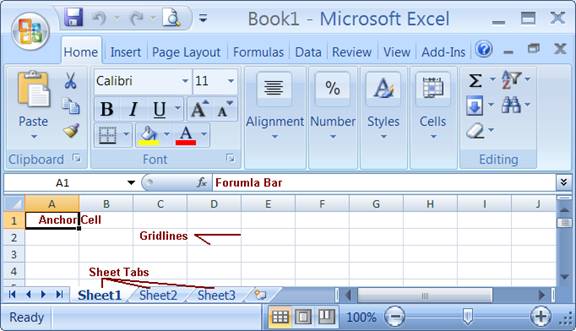
Title Bar - is something that you have seen before. Remember the title bar shows you the name of the application that you are using (Microsoft Excel) and the name of the file, Book1[3].
Formula Bar - will display what is actually typed into the cell. In the case of a formula or function it will display the actual formula in the formula bar. The result would be displayed in the cell.
Sheet Tabs - identify the sheet you are working on. In some spreadsheets you have one sheet per file. In Excel and other spreadsheets you can have several sheets all in one file. It all works the same as dealing with one sheet for the most part. As you learn more advanced spreadsheet topics you will discover some advantages to having more than one sheet in a file. Sheet tabs can be named by double clicking the sheet tab. Sheet is the default name.
Gridlines - are the light gray lines that outline the rows and columns. These can be turned on or off.
End of Document in a spreadsheet - There is no end of document marker in the spreadsheet but you can find the end by pressing Ctrl + End. This will take you to the cell that the computer thinks is your last one. You may find that you have several empty columns or rows (they should not print). I have not had much luck in getting rid of them.
Creating a new spreadsheet
When you start Excel it will automatically start a new spreadsheet file with 3 sheets (remember the sheet tabs are at the bottom). Your cursor should be on cell A1. Your first step in creating a new spreadsheet actually begins on paper. You should write down a rough outline of how you want your spreadsheet to look. You should include in your outline the following:
1. Rough draft of how it should look, something like sown in Figure 5.
2. Sample numbers.
3. Formulas with the expected results, given the sample numbers.
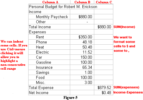
Now that we have a picture of what it is we want to do it will be easier. I have listed all my known expenses as well as my income. I know that my net income is any money that I have left over. I get net income by subtracting my total expenses from my total income. I have even included a bunch of formatting features as well such as dollar signs, commas and decimal places. Now before we begin we should save our new document.
Saving a document
Just like in word processing you should save your document
before you begin and then many times as you work so that you do not lose any
information. Saving a file in a spreadsheet is exactly the same as in the word
processor. Choose Office Button, Save As... ![]() and name your file with a name that will make
sense to you. Be sure to save the file in the correct folder as well. In this
case I will name the file BUDGET. As
with the word processor, an extension will be placed on the end automatically.
In the case of Excel it will be XLSX.
Now that your file is saved, be sure to use
and name your file with a name that will make
sense to you. Be sure to save the file in the correct folder as well. In this
case I will name the file BUDGET. As
with the word processor, an extension will be placed on the end automatically.
In the case of Excel it will be XLSX.
Now that your file is saved, be sure to use ![]() Save periodically
to save the changes that you make.
Save periodically
to save the changes that you make.
Simple Formulas
The beauty of spreadsheets is the ability to create formulas. Well not so much create formulas but that the results will be automatically recalculated each time you change one of the numbers. When you create a formula you should do two things:
1. Know what the answer will be by figuring it out on paper first.
2. Use cell references so that you can change the numbers in the formula and see how the result will change.
Doing your formula on paper first is a simple testing method that is used in computer programming many times. When you type a formula into a spreadsheet it will display the result of that formula when you hit enter. This result may be right or it may be wrong. What I mean is the computer will calculate the formula correctly, however you may type in the wrong formula. If you do the formula on paper first, including writing down the answer, you will know if you have entered your formula in correctly.
In our example our only formula is calculating our Net Income. This is done by:
Net Income = Total Income - Total Expenses
Putting this into spreadsheet terminology we need to replace the words, with cell references. In other words what cells do the numbers come from? Let’s look at the sample spreadsheet that we are going to make. I have indicated what the columns are going to be so we only need to count down the rows. We will assume that we are starting in row 1. Therefore Total Income will be located in cell C5. Total Expenses will be in cell C17. The actual formula will go into cell C18. So on paper we would write this down like shown below (what you actually type into the cell would be =C5-C17):
Net Income = Total Income - Total
Expenses
C18 = C5 - C17
When we write out our formulas in this manner; first in English then in spreadsheets format, we begin to learn the step by step design commonly used in computer programming. This is a great way to document the spreadsheet on paper in case we have to come back and fix it later[4].
As your formulas get more complicated you want to remember the order of evaluation: Parenthesis, Exponents, Multiplication, Division, Addition, and Subtraction. It is always better to use Parenthesis so that the formula is easier to read.
Simple Functions
A function is a built in formula that comes with the spreadsheet program. These are commonly used formulas. They consist of the function name followed by the parameters or arguments enclosed in parenthesis. If there is more than one argument each will be separated by a comma. As with formulas all functions must begin with an = sign[5].
Our first function will be the SUM function which is used to add up a range of numbers. The syntax of the SUM function looks like this:
SUM(range)
where the range is the range of cells that you want to add together. Simply put, the SUM function will add the range of cells together. A few more simple functions are MIN(range), MAX(range), and AVERAGE(range). These are all pretty self explanatory as they will find the smallest number in the given range, the largest number in the given range and the average of all the numbers in a given range. I may use these functions in looking to see what the lowest grade was on an exam. Likewise I would be interested in the highest grade as well as the average grade.
Absolute and Relative Cell Addresses
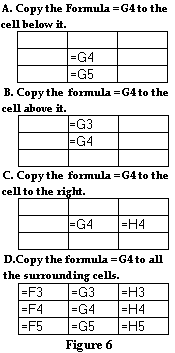 A nice feature of spreadsheets is their
ability to change a formula (or function) when you copy the formula to another
cell. For example, if you have the formula =G4 located in a cell (it does not
matter which one) and you copy that formula (Edit, Copy) to the cell below it, the formula will
change to =G5 Figure 6A. If you copy the formula to the cell above, the
formula will change to =G3 Figure 6B. Likewise if you copy the formula to
the cell on the right it will become =H4 Figure 6C. This is because =G4 is
a relative
cell reference, meaning it will change relative to the cell
you copy it into. Most of the time this is what you want it to do. As you can
see in Figure 6D your formula will change no matter where you copy it to.
A nice feature of spreadsheets is their
ability to change a formula (or function) when you copy the formula to another
cell. For example, if you have the formula =G4 located in a cell (it does not
matter which one) and you copy that formula (Edit, Copy) to the cell below it, the formula will
change to =G5 Figure 6A. If you copy the formula to the cell above, the
formula will change to =G3 Figure 6B. Likewise if you copy the formula to
the cell on the right it will become =H4 Figure 6C. This is because =G4 is
a relative
cell reference, meaning it will change relative to the cell
you copy it into. Most of the time this is what you want it to do. As you can
see in Figure 6D your formula will change no matter where you copy it to.
There are times when you do not want the formula to change. This is when you would use an absolute cell reference . An absolute cell reference does not change when you copy it. To make a cell address absolute you need to include a $ sign like this: =$G$4. If we copy =$G$4 to the cell below it, the formula will still be =$G$4 no matter what.
You can also have what is called a mixed cell reference. This is where half of the formula will change when you copy it. For example: =$G4 means that the column($G) is absolute but the row(4) is relative. If you copy this to the cell below it will become =$G5. Now if you copy =$G4 to the cell to the right it will still be =$G4. You do not use mixed cell references that often.
Now if you never
need to copy formulas it does not matter, but when building a spreadsheet it is
often handy to know the difference between the two main types. Looking at the
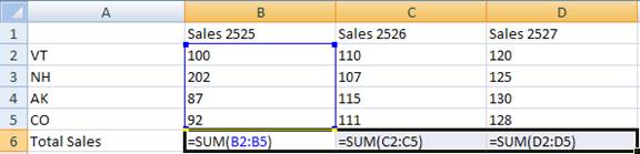
sample spreadsheet in Figure 7, you can see that I am using the sum function
to total the three columns individually. Now if I use relative cell addresses I
can copy =SUM(B2:B5) to the cell next to it and following the rules of relative
cell address it will become =SUM(C2:C5). If I did not want the formula to
change I would use an absolute cell address. In Figure 7 I am causing the
computer to display the formulas in the spreadsheet instead of the numbers.
Look for show formulas icon ![]() on the Formulas
tab, Formulas Auditing group.
Displaying formulas will change your column widths. Your column widths will
change back when you turn the option off. You may just want to save the
document first.
on the Formulas
tab, Formulas Auditing group.
Displaying formulas will change your column widths. Your column widths will
change back when you turn the option off. You may just want to save the
document first.
It can be difficult at first to decide which to use; absolute or relative. In the beginning you will often just use relative cell address and copy the formula. If it does not come out right just go back and change it to absolute and copy it over again. As a very general rule if you are using cell references on the same row you will want to use relative. If you are going to use the same cell reference in more than one formula you will want to use absolute. You can have an absolute cell reference and a relative cell reference in the same formula.
Fill Right, Fill Down
We
can actually use a feature called Fill
Right to copy the SUM function from cell B6 to C6 and D6. What you do is
type in the function in cell B6 and then click and drag on the fill handle ![]() to cell D6. This feature will take the
contents of the anchor cell and copy it to the highlighted cells. This is the
same as choosing copying and pasting, you are just able to do all the cells at
once. In the case of text, it will just copy the text in the anchor cell to the
highlighted cells. In the case of the function it will copy the function (or
formula) to the highlighted cells. If you use relative cell references they
will change like they are supposed to.
to cell D6. This feature will take the
contents of the anchor cell and copy it to the highlighted cells. This is the
same as choosing copying and pasting, you are just able to do all the cells at
once. In the case of text, it will just copy the text in the anchor cell to the
highlighted cells. In the case of the function it will copy the function (or
formula) to the highlighted cells. If you use relative cell references they
will change like they are supposed to.
You can use the Fill Handle to Fill Down as well and it works the same way only you highlight down in a column instead of across in a row. These are very handy features to keep in mind when building your spreadsheet.
 Insert Row or Column
You
may find that you need to insert a new row or column in an existing
spreadsheet. The rule to follow is that the row will be inserted above the cursor and the column will be
inserted to the left of the cursor.
So you simply place the cursor in the correct location and choose Insert, found on the Cells Group on the Home Tab. If you need to
insert more than one simply highlight the number you need to insert first. The
same rule applies above or to the left of the cursor.
Just because you have inserted a new column does not mean that you actually have more columns. A spreadsheet has 256 columns. When you insert a column you STILL have 256 columns. You actually move the columns over one. The same holds true for rows.
Page Setup
There are several neat options available to us in Page
Setup. The first tab I want to talk about is Page. Choose the Page Layout Tab, Page Setup ![]() to get the dialog box shown below.
to get the dialog box shown below.
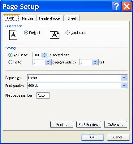
This is the place to set the spreadsheet’s orientation by simply choosing the correct option button. The only new feature here is the scaling section. You can have your document Fit to the page. This will shrink the document to fit in the number of pages that you have specified. With the Print Preview button handy you can simply check it out to see if you like the way it looks. If you do not like the way it looks choose the Setup... command button in print preview to get you back to the above dialog box. Also notice that this is the place to set your First Page Number (currently set to auto).
 Margins
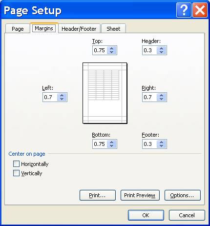
Still in the same dialog box we can adjust our margins by clicking on the margins tab Figure 11. You can also use the margin icon found in the Page Layout Tab. You set margins in the same way that you did for word processing. They will apply to the entire Sheet. Each Sheet can be set differently. The only new option you have is the ability to center the spreadsheet on the page, both Horizontally and Vertically by clicking the appropriate check box. The sample Preview section will show you what it will look like.
Print..., Print Preview and Options Command Buttons are just fast ways to print the file, preview the file or change printer options. The Help command button will give you help information about the Header/Footer dialog box. OK will accept the information and Cancel will just leave everything the way it was.
Headers & Footers
Moving to the next tab in the same dialog box, Header/Footer tab Figure 12 it looks a little different than in the word processor, but the concept is the same where a header shows up at the top of every page and the footer shows at the bottom of every page.
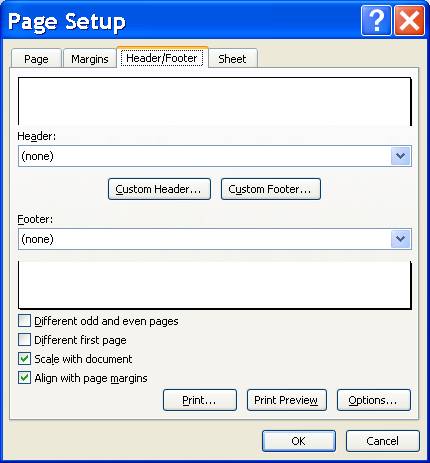
If you choose the Header List box you will see several pre-made headers that you can use. If you see one that you like you can simply click on it. Header and footers work the same way so I will just explain headers.
Now if you choose Custom Header... you will get a dialog box that looks like Figure 13.
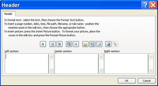
 You have three sections that you can put
information into. These sections are basically the Left Section that will be left aligned on the left margin.
The Center Section to have
the text centered between your margins and the Right Section that will be right aligned on the right
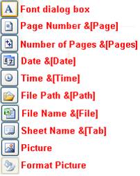
margin. There is a code in the center section that stands for the name of the Sheet Tab. You can insert several different codes into the header or
footer section. You can delete the &[Tab] if you do not want it. You can
place the codes in any section. If one section is too long it will simply
continue into the next section. For example: if your left section is long it
will go into the center section. If you have anything in the center section it
will go over the top of it and print both sections. Check print preview to see.
You can have different fonts in a section if you want. It is common to have the
header and footer a smaller size font than the spreadsheet (just like in word
processing).
You have three sections that you can put
information into. These sections are basically the Left Section that will be left aligned on the left margin.
The Center Section to have
the text centered between your margins and the Right Section that will be right aligned on the right
margin. There is a code in the center section that stands for the name of the Sheet Tab. You can insert several different codes into the header or
footer section. You can delete the &[Tab] if you do not want it. You can
place the codes in any section. If one section is too long it will simply
continue into the next section. For example: if your left section is long it
will go into the center section. If you have anything in the center section it
will go over the top of it and print both sections. Check print preview to see.
You can have different fonts in a section if you want. It is common to have the
header and footer a smaller size font than the spreadsheet (just like in word
processing).
Sheet
The last tab in the Page Setup Dialog box deals with the sheet as shown below.
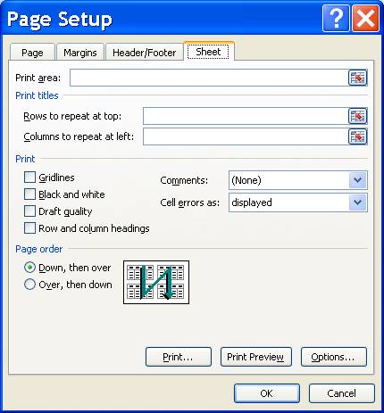
The Print Area is for you to specify a range of cells that you want to print. This way you do not have to print an entire spreadsheet. Often times a spreadsheet will have tables and sections that are used for calculating and you only want to print a certain range. To do this place your cursor in the Print Area text box and type in the cell range. If you do not remember simply click on the spreadsheet and highlight the area with the mouse. This will place the cell range in the text box for you.
There is a menu option File, Print Area …, that gives you the options to Set Print Area or Clear Print Area. To set the print area this way you simply highlight what you want to print and then choose, File, Print Area…, Set Print Area. After printing you may want to reset the print area back to what it was so you can then choose the Clear Print Area option.
Normally when you print, the computer will print out all the cells that you have information in. This will be an area in a range that the computer assumes that you have used. There will be blank cells of course. Basically it will print the farthest column that you have information in and up to the last row that you have information in.
Print Titles are
used to repeat a column or row title on each page. For example you are printing
a large table that will take two pages to fit. The second page will have a
bunch of numbers but no column labels to tell you what those numbers are for.
Looking 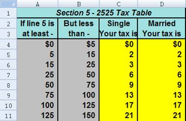 at the tax table shown, this table is
large. It goes all the way to row 1066 and takes about 30 pages to print. Now
when we are looking at page 25 you may forget what the numbers in each column
stand for. We would like rows 1, 2 and 3 to show up on each page. So we can
type the range 1:3 in the Rows to
Repeat at top text box or we can use the mouse to highlight
the three rows. If we want to repeat columns we would do the same thing only
specify which columns we want to show up on each page.
at the tax table shown, this table is
large. It goes all the way to row 1066 and takes about 30 pages to print. Now
when we are looking at page 25 you may forget what the numbers in each column
stand for. We would like rows 1, 2 and 3 to show up on each page. So we can
type the range 1:3 in the Rows to
Repeat at top text box or we can use the mouse to highlight
the three rows. If we want to repeat columns we would do the same thing only
specify which columns we want to show up on each page.
In the Print section I only want to cover two check boxes, Gridlines and Row and Column Headings. Sometimes you want the gridlines to show on the printed copy and other times you want to have borders show instead. You can turn the gridlines on or off by clicking the check box. The Row and Column headings are handy to print when you want to be able to see on paper what the cell coordinates would be. Again it is a simple matter of checking the check box. For all the other options simply choose help to learn more about them as at the moment they go beyond the scope of the course.
Formatting
 Most
of the formatting features all work the same as they did in the word processor.
Bold, Italic, Underline, Left Aligned, Right Aligned, Center Aligned, Borders, Shading, Font, and Size all
work the same except that they affect the entire cell instead of a single
character or paragraph. In other words the entire cell would be in bold, or the
cell contents would be centered in the cell. If you highlight one word in the
formula bar then only that word would be bold. By default the spreadsheet
assumes you want the entire cell formatted. All of these are available from the
Home tab, Font Group.
Most
of the formatting features all work the same as they did in the word processor.
Bold, Italic, Underline, Left Aligned, Right Aligned, Center Aligned, Borders, Shading, Font, and Size all
work the same except that they affect the entire cell instead of a single
character or paragraph. In other words the entire cell would be in bold, or the
cell contents would be centered in the cell. If you highlight one word in the
formula bar then only that word would be bold. By default the spreadsheet
assumes you want the entire cell formatted. All of these are available from the
Home tab, Font Group.
An alignment feature we have not discussed yet is center across selection and this will center the cell contents in the highlighted selection. You simply highlight the range of cells that you want to center a particular text on (i.e. columns A, B, and C) and choose the center across selection button on the toolbar or choose Format, Cell..., Alignment, Center Across Section. You should have the text in the first cell.
There are some
formatting features specific to spreadsheets Figure 17 and they are number
formats. These include currency, comma and percent format features. You
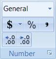 can
also specify the number of decimal places for each of these. Just remember that
if you do not want any decimal places than set the
can
also specify the number of decimal places for each of these. Just remember that
if you do not want any decimal places than set the 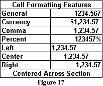 decimal places to zero. You can do this all
from the Home tab, Number Group.
decimal places to zero. You can do this all
from the Home tab, Number Group.
General format is the
default format. Each of these cells Figure 17 has exactly the same number
in them, 1234.567. So we can see the effect that each feature has. When I have
used a decimal, I have rounded the number to 2 decimal places. You can increase
or decrease ![]() the number of decimal places.
the number of decimal places.
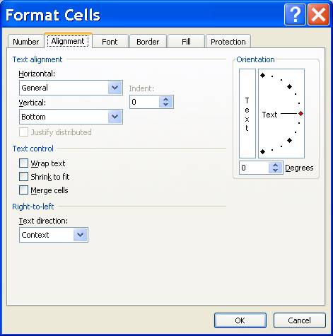
Most of the formatting features should actually be under the same menu as they were in the word processor. Looking at the Figure above is the dialog box found in the Home Tab, Cells Group, Format, Format Cells..., we can see all the features that we can do.
Number - holds all the different number formats that you can choose from. You can also create your own custom number style (refer to help).
Alignment - is the different ways that you can align the information in your cells. The common ones are left, center, and right. There is also center across selection as well as horizontal and vertical alignment features. Notice the wrap text check box (allows for two lines in the same cell). The Orientation is a funky feature, check it out.
Font - holds all the same things that it did in the word processor.
Border - allows you to place a border around the cell or highlighted range. You can specify several styles as well as sides. Each side can be different. Oh, don’t forget about color! Combined with a pattern you can really direct attention to particular cells.
Patterns - allow you to shade or color a cell background. It is called Shading in the word processor.
Protection - allows you to protect a cell from accidentally deleting the contents. More on this in the next chapter.
Column Width
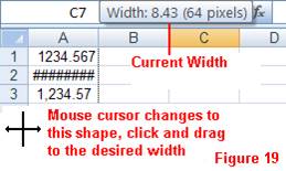 Often
you will need to change the width of a column (row height can also be changed).
The easiest way to change to the column width is to use the mouse and drag the
column to the size that you want Figure 19. A double click action will
result in the computer choosing a best fit. The computer will choose a
size that should fit all the cells in that column. Sometimes this does not
work, be sure to check print preview. If you are having trouble setting the
width with your mouse, choose Home Tab, Cells
Group, Format and choose the option you need from the drop down menu.
Often
you will need to change the width of a column (row height can also be changed).
The easiest way to change to the column width is to use the mouse and drag the
column to the size that you want Figure 19. A double click action will
result in the computer choosing a best fit. The computer will choose a
size that should fit all the cells in that column. Sometimes this does not
work, be sure to check print preview. If you are having trouble setting the
width with your mouse, choose Home Tab, Cells
Group, Format and choose the option you need from the drop down menu.
Freeze Columns or Rows
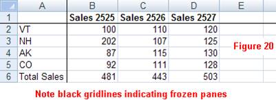 There
are times when you want a column or two to always be on the screen at all
times. You may have column (or row) headings that identify the numbers. When
you scroll over a few columns you can no longer see those headings. You can
FREEZE the headings so that they do not scroll. This is very similar to Print
titles only they affect just the screen display. You place the cursor where you
want to Freeze the column (or row) and choose View Tab, Windows Group, Freeze Panes, Freeze Panes. This will freeze the columns to the left of the cursor and the rows above the cursor. To get rid of frozen
panes (warm them up, just kidding) you should notice that Freeze Panes changes to Unfreeze
Panes. When panes are frozen there will be a
solid black gridline showing you the frozen panes. In Figure 20 I have
frozen row 1 and column A, then I scrolled over a column.
There
are times when you want a column or two to always be on the screen at all
times. You may have column (or row) headings that identify the numbers. When
you scroll over a few columns you can no longer see those headings. You can
FREEZE the headings so that they do not scroll. This is very similar to Print
titles only they affect just the screen display. You place the cursor where you
want to Freeze the column (or row) and choose View Tab, Windows Group, Freeze Panes, Freeze Panes. This will freeze the columns to the left of the cursor and the rows above the cursor. To get rid of frozen
panes (warm them up, just kidding) you should notice that Freeze Panes changes to Unfreeze
Panes. When panes are frozen there will be a
solid black gridline showing you the frozen panes. In Figure 20 I have
frozen row 1 and column A, then I scrolled over a column.
Spell checker
You can check the spelling in your spreadsheet the same as you did in the word processor the icon is found under the Review Tab. If you highlight a range of cells then only those cells will be checked for spelling. Refer back to Chapter 1 for more information on the spell checking module if you need to.
What’s Wrong with these functions /spreadsheets
=SUM(A1-B1) is wrong because sum is a function to add not to subtract. It should simply be =A1-B1.
=A1+B1+C1+D1 is okay (it would be marked wrong on an assignment) but it is more efficient to use the sum function =SUM(A1:D1).
=SUM(A1:D1)*=MIN(G6:H6) is wrong because the second equal sign is incorrect, you only need to start a formula with one equal sign. The correct formula that combines two functions would be: =SUM(A1:D1)*MIN(G6:H6).
 =A1*B1+B2*C3
is wrong because in this case we want to multiply A1 times B1 + B2. That is not
how this will work. It will multiply A1*B1 and multiply B2*C3 and then add
those two values together. The way it should be written is like this using
parenthesis: =A1*(B1+B2)*C3.
=A1*B1+B2*C3
is wrong because in this case we want to multiply A1 times B1 + B2. That is not
how this will work. It will multiply A1*B1 and multiply B2*C3 and then add
those two values together. The way it should be written is like this using
parenthesis: =A1*(B1+B2)*C3.
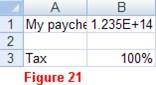
Looking at Figure 21 we can see a couple of mistakes. The first one is that we need to increase the column width for column A. Text in a cell will flow into the next cell only if the next cell is empty. Now cell B1 has a groovy little number that I really wish was my paycheck! This is in exponential form. What you would need to do is to format this cell for comma or currency notation. You will most likely have to increase the column width when you do so that the number will be more readable. We all know it seems like the government gets 1000% of our paychecks for taxes but in this case I typed in 10 instead of .10 for ten percent. Remember that when using the percents you need to move the decimal place.
 Look
at Figure 22. Besides the fact that I am never going to be able to save up
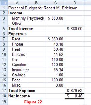
for a house on this budget, what can you see that is wrong? Well column B is
blank. This would cause us a problem if we were to graph our expenses later on.
We should delete column B, this should automatically readjust our formulas but
if not just redo them.
Look
at Figure 22. Besides the fact that I am never going to be able to save up
for a house on this budget, what can you see that is wrong? Well column B is
blank. This would cause us a problem if we were to graph our expenses later on.
We should delete column B, this should automatically readjust our formulas but
if not just redo them.
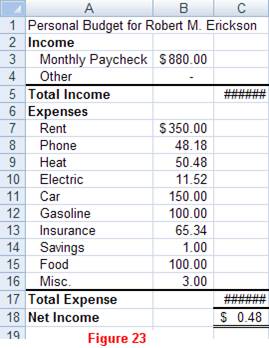
Well I fixed the blank column and the spelling errors but in Figure 23 I ran into a problem, re-sizing my column widths. What happened to column D? When you see a series of # signs in a cell it simply means that the column is not wide enough and you need to enlarge the column width for that column. In this case enlarge column D until the # signs disappear. You will want to check Print Preview before you print. On occasion I have seen the # signs in Print Preview but not when looking at the document. Nothing to worry about. Simply close the Print Preview and make the column a little larger. Check Print Preview again to see if it is fixed.
 In
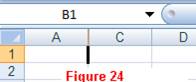
Figure 24 you will notice that column B is missing! When I was adjusting
the column (B) I accidentally set the width to zero. To fix this we need to GO
TO column B and then use Format Column
Width to fix it. If you press the F5 key (No idea what the icon is for
this) it will ask you what cell to go to. Type in B1. Now choose Format Column Width (Home Tab) and set
the width to something greater than zero.
In
Figure 24 you will notice that column B is missing! When I was adjusting
the column (B) I accidentally set the width to zero. To fix this we need to GO
TO column B and then use Format Column
Width to fix it. If you press the F5 key (No idea what the icon is for
this) it will ask you what cell to go to. Type in B1. Now choose Format Column Width (Home Tab) and set
the width to something greater than zero.