Chapter 5 Spreadsheet Functions
Contents
Chapter 5 Spreadsheet Functions
Referring
to cells in a different sheet..
What’s
wrong with this function
Spreadsheet Functions
 There are
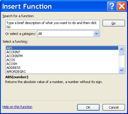
several hundred functions available to you in a spreadsheet. The easiest way to
learn all of them is to choose the
There are
several hundred functions available to you in a spreadsheet. The easiest way to
learn all of them is to choose the ![]() Sum
Icon to get the drop down menu of the most common functions and choose More Functions … at the bottom
of the list. This should give you an alphabetical listing of all the functions
(you may need to select change the category to All. All functions have a function name followed by the parameters
(arguments) of the function. Some parameters are simple like a cell range;
others are more complex like a logical condition, action for true condition and
action for false condition. Functions are really built in formulas. In other
words for each function there is a mathematical formula that will do the same
thing. However the formula is usually long and complicated so the makers of the
spreadsheet have provided you with functions to simplify the process.
Sum
Icon to get the drop down menu of the most common functions and choose More Functions … at the bottom
of the list. This should give you an alphabetical listing of all the functions
(you may need to select change the category to All. All functions have a function name followed by the parameters
(arguments) of the function. Some parameters are simple like a cell range;
others are more complex like a logical condition, action for true condition and
action for false condition. Functions are really built in formulas. In other
words for each function there is a mathematical formula that will do the same
thing. However the formula is usually long and complicated so the makers of the
spreadsheet have provided you with functions to simplify the process.
The easiest way to do any function is to write the function and all the parameters out by hand first. I will describe how to do this with the PMT function.
PMT Function
The PMT or Payment function can figure out what your monthly payment on a loan will be, given the interest rate, the number of payments and the principal amount. Let’s look at the arguments for this function and talk about them for a moment.
=PMT(rate,
nper, pv, fv, type)
rate is the interest rate for your loan.
nper is the number of payments you will be making.
pv is the present value or the principal amount of your loan.
fv and type are not required parameters. We will not use them for now.
As always in order to get a complete description of the PMT function simply use help and search for it. One important thing to note is that I have already read the help so I know that if I want to have monthly payments I need to make sure the rate and nper are both in months. The interest on most loans is quoted as an annual interest rate. Since nper is the number of monthly payments that you want to make, you need to adjust the annual interest rate to a monthly one by simply dividing the rate by 12.
Following the basics of spreadsheets I want to use cell references for my functions whenever possible. I also want to write it out on paper first since it will make it easier. Figure 1 is how I want my spreadsheet to look:
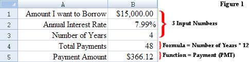
Remember the four things a computer can do input, processing, output and storage. In our case here you can see the input numbers, the function itself is the processing and the output is our monthly payment displayed on the screen. I have used a simple formula to calculate the total payments by taking the number of years and multiplying by 12. Or in spreadsheet language =B3*12 is the formula located in cell B4. Now let’s figure out the PMT function. The first step is to put it all on paper like this:
=PMT(rate, nper, pv, fv, type)
rate - is our annual interest rate or .0799 (7.99%) remember that when you take the % sign off you need to move the decimal point 2 places to the left. We also need to divide this by 12 so to get the monthly interest rate, .0799/12.
nper - is the number of payments that we want to make. We want a 4-year loan so that would be 48 payments.
pv - is the principal amount of our loan or 15000. We do not want to use commas when writing this number since the computer would think that we are separating parameters.
Note: The payment function will return a negative number. Now we could plug in the actual numbers to come up with the function like this:
=PMT(.0799/12,48,15000)
Now this would work but it is not very flexible. If we wanted to change the amount, the term, or the interest we would have to edit the function. When you use cell references you can simply type the number in the correct cell.
Once you figure out the function in ‘English’ like we did above, you need to then convert your English into spreadsheet. So let’s do that now:
=PMT(rate, nper, pv, fv, type)
rate -.0799/12 - We find the interest rate in cell B2 so let’s write the rate as B2/12
nper - 48 payments can be found in cell B4.
pv - 15000 - We can find the principal in cell B1 B1
=PMT(B2/12,B4,B1)
If you want the display to be positive you can use the ABS (Absolute Value) function like this:
=ABS(PMT(B2/12,B4,B1))
Now we can simply change the amount we borrow, the interest rate or the number of years for our loan in the correct cell and automatically come up with our new monthly payment. So now you can put in the amount of that new car you want and get a rough idea of how much it will cost you. Can you develop the formula to tell you how much you will actually have to pay the bank[1]? How much in interest will you pay on this loan[2]?
Developing your functions (or formulas) in this step by step approach helps you develop the logical thinking required for more complex problems. So in addition to learning functions you are also using a problem solving step by step approach.
VLOOKUP Function
 The
VLOOKUP or Vertical Table Lookup function will search a table for a specified
number and return a number for you. An example would be a sales tax table like
Figure 2. If you make $1 purchase in
The
VLOOKUP or Vertical Table Lookup function will search a table for a specified
number and return a number for you. An example would be a sales tax table like
Figure 2. If you make $1 purchase in
VLOOKUP(lookup_value, table_array, col_index_num, range_lookup)
Lookup_value is the value that you are going to look up in your table. In the sales tax example it will be our purchase amount or $1. The computer will always look for the value in the first column of your table only.
Table_array is the cell range that your table is in. This would start from the first column, first row ($0.00) and go to the last column, last row (0.05). You do not include the labels, only numbers. Naturally you would need to use cell references.
col_index_num is the column number that contains the information that you are looking for. In the sales tax table we are looking for the sales tax that is located in column two, so our column index number is 2. Column A, Column B is not what is meant by the Column Index Number. Instead the first column in your table range is column 1, the second column in the range is column 2.
range_lookup is an optional parameter that is used if your first column is not in ascending sorted order (1,2,3). When not specified it is set to TRUE. If for some reason your first column of your table is not in sorted order you can set this parameter to FALSE. In the case of TRUE, VLOOKUP will return a value that is equal to or the next largest value that is less than the lookup_value. In the case of FALSE the lookup_value must match exactly.
If VLOOKUP can't find the lookup_value, and range_lookup is TRUE, it uses the largest value that is less than or equal to lookup_value. In other words it will always take your lookup value and round it down. If lookup_value is smaller than the smallest value in the first column of table_array, VLOOKUP returns the #N/A error value. So if your lookup value is too small (in the example less than 0) the computer will let you know, however if the value is too large (greater than 1.09) it will just give you the last number in the table. For example if your purchase amount is $10, the VLOOKUP will return a 0.05 sales tax! That is just the way it works.
If VLOOKUP can't find lookup_value and range_lookup is FALSE, VLOOKUP returns the #N/A value. This is because the FALSE value says the lookup_value must match the table exactly.
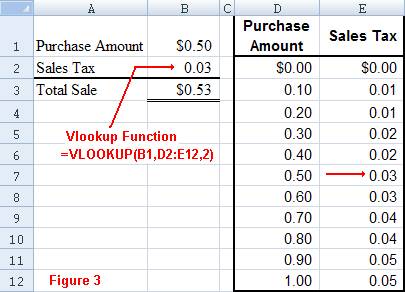
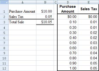
Looking at Figure 3 we would place the VLOOKUP function in cell B2, to find the tax on our purchase amount in cell B1. AS the arrow points the VLOOKUP returns the 0.03 sales tax.
Thus writing our VLOOKUP function out on paper it would look like this:
VLOOKUP(lookup_value, table_array, col_index_num, range_lookup)
lookup_value is our purchase price
B1
table_array is the cell range our table is located in
D2:E12
col_index_num will be 2 since we want to display our sales tax.
Now putting all this together our VLOOKUP function would look like this:
VLOOKUP(B1,D2:E12,2)
Let’s look at a couple of samples:
Our Purchase Amount VLOOKUP will return
< 0 NA
> 1 0.05
0.40 0.02
0.85 0.04
1.00 0.05
1.10 0.05
50.00 0.05
What would the sample spreadsheet display if we changed the column_index_num to 1? Currently it is set to 2 and with a purchase amount of $ 0.50, our sales tax is 0.03. If we change the column_index_num number to 1 it would simply display 0.50 which is in the first column.
IF Function
The IF function is used when you want to display one of two possible answers. In other words an IF function is a question that has a yes or no answer. You then can display one number if the question is answered yes, or a different number if the answer is no. Let’s look at the parameters of the IF function:
IF(logical_test, value_if_true, value_if_false)
logical_test - is the yes/no question. An example would be “Is
hours worked greater than 40”? This is a question that will have a yes or no
answer. In spreadsheet terms it would look like C3>40 (providing C3 contains
the hours worked).
value_if_true - is the action that you are going to take if the answer is yes (true). Now the action can be a number, a label, another function or even a formula. Some examples would be:
display some text - “Overtime!”
display a cell contents - B3.
Calculate regular pay as 40 times pay rate - 40*B3 (assuming B3 holds the pay rate).
Calculate overtime pay as (hours worked - 40) times pay rate times time and a half - (C3-40)*B3*1.5. Notice the use of parentheses in this case to ensure that I perform the subtraction first.
value_if_false - is the action that you are going to take if the answer is no (false). The action can be the same as any examples that I used for value if true. Sometimes you may want to do nothing. An example of a do nothing action would be:
display zero - 0.
display nothing - “”
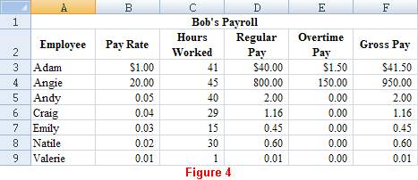
Let’s figure out a couple of IF statements. An easy one, is to use a spreadsheet to calculate regular pay, overtime pay and total pay. In order to do this we will need to have for input, the hours worked and the pay rate. We will assume an overtime rate of time and a half. Let’s look at the sample spreadsheet in Figure 4 and prepare our functions by hand. One thing that you may want to do is to use easy numbers. For example I may pay people (like Angie) $20 per hour (they wish) but if I use a $1 hour pay rate like I pay Adam it will be very easy for me to calculate the answers. I know regular pay will be $40 and overtime pay will be $1.50. The multiplication is just easier.
Let’s start with the formulas for Adam and figure Regular Pay for cell D3. You need to use the if statement:
IF(logical_test, value_if_true, value_if_false)
logical_test our logical test is going to be did they work over
40 hours or is hours worked greater
than 40? In a spreadsheet it would
read
C3>40
value_if_true would be yes they did, so regular pay is going to
be for 40 hours or 40 times their pay rate.
40*B3
value_if_false would mean they did not work more than 40 hours
therefore regular pay would be the hours
they worked times their pay rate
C3*B3
Put all that together in the IF statement for cell D3 (Regular Pay) will look like this:
=IF(C3>40,40*B3,C3*B3)
Looking at the IF statement is confusing to me but if we work out the function in English first, it really is not that hard. Let’s try Overtime Pay as it can be a little harder. I am going to change the wording of the parameters and give the commas a word. Maybe the IF statement will make more sense to you this way in Figure 5. The parameters are still the same only worded differently. You may want to substitute this wording if you find it easier.
The short cut that I use to write this statement is
=if(?,Y,N). Now let’s work on the formula for overtime pay in cell D3.
Question (logical_test)
our logical test can be the same, did they work over 40 hours or is hours worked greater than 40?
C3>40
Yes its true (value_if_true) would be yes they
did, so we need to pay them for the hours they worked over 40 times time and a
half. An easy way to do this is to figure the hours times the pay rate
times 1.5.
(C3-40)*B3*1.5
No it’s false (value_if_false) would mean they did not work
overtime and should not get any overtime pay so it should be 0.
0
Put all that together in the IF statement for Overtime pay in cell E3 will look like this:
=IF(C3>40,(C3-40)*B3*1.5,0)
=IF(
? , Y ,N)
Again it is easier to write the statement out in ‘English’ first and then convert it to spreadsheet IF function. The gross pay is simply a sum function adding regular pay and overtime pay.
Let’s do all the same formula for Angie’s Regular pay in cell D4:
IF(logical_test, value_if_true, value_if_false)
logical_test is hours
worked greater than 40
C4>40
value_if_true 40
times their pay rate.
40*B4
value_if_false hours
they worked times their pay rate
C4*B4
Put all that together in the IF statement for regular pay in cell D4 will look like this:
=IF(C4>40,40*B4,C4*B4)
 Not much difference is there? Only the
row numbers change. Does that sound like we can copy the formula for all the
employees? Yes we can, and since we are using relative cell address they will
automatically change. In fact all the formulas in Figure 4 can be copied
down to the next row. There is an easy way to do this and that is to highlight
from D3 to F9. We can use fill down (See Chapter 4) which is a very handy
feature. Since we used relative cell references they automatically will change.
Not much difference is there? Only the
row numbers change. Does that sound like we can copy the formula for all the
employees? Yes we can, and since we are using relative cell address they will
automatically change. In fact all the formulas in Figure 4 can be copied
down to the next row. There is an easy way to do this and that is to highlight
from D3 to F9. We can use fill down (See Chapter 4) which is a very handy
feature. Since we used relative cell references they automatically will change.
Nested If Statement
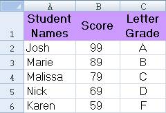
Let me give you an example of a nested if statement (2 ifs in one formulas). As always I want to start simple. Looking at Figure 6 cell B2 holds a students total points. What I need is a formula to display the student’s final letter grade. So, let's make this simple, in my class I give 2 grades, A or F (hey that sounds like a good idea!). If your total score is greater than 89 you will get an A else you will get an F. I start by writing out the parameters of the IF statement. I am going to use my little shortcuts this time:
=IF(?,Y,N)
my question is going to be:
? is total score > 89
in spreadsheet format this will be:
B2>89
If the answer to that question is yes then:
Y "A"
And if the answer to that question is no then:
N "F"
Putting that all in one statement:
=IF(B2>89,"A","F")
Okay so maybe that would make it easier for me to figure out the final grades but I think that maybe we should at least give people a "B" if they get a score greater than 79. So what we have now is:
If your grade is greater than 89 you will
get an A else
If your grade is greater than 79 you will
get a B else
You will get an F.
You should notice that the first part of the formula will stay the same. What we need to do is change the "F" (I hear that one all the time!). So on paper we have something like this:
IF(
? , Y , N )
?
Score > 89
B2
> 89
Y
"A"
N IF(
? , Y , N )
?
Score > 79
B2
> 79
Y
"B"
N
"F"
Putting that all into one statement we get:
=IF(B2>89, "A", IF(B2>79, "B", "F"))
Make sense to you? I also suggest that you type the formula in one step at a time so that you can be sure each step is working. Looking at our formula I suppose we really need to add the letter grades C and D. Eventually we would get the complete formula like this:
=IF(B2>89, "A", IF(B2>79, "B", IF(B2>69, "C", IF(B2>59, "D", "F"))))
Cool. I wonder if we should do the + and - grades as well? Go for it, it just makes one very long nested IF formula! I know because I have typed it in to help me calculate the final grade for everyone.
Combining Functions Together
You can have an IF statement inside of another IF statement as the Value_if_true. This would be called a nested IF. You can also combine VLOOKUP and IF together. When you combine functions it is really not any harder than doing them one at a time. Remember to write the whole thing out on paper first and you will be able to understand it easier.
Let’s try to combine an IF and VLOOKUP together to see how this would work. Remember that if the VLOOKUP statement tried to look up a number that was too large for our table it would just use the last number. Looking at our tax table in Figure 7 we see if our purchase price was $10.00, we would need to use a different table, however the VLOOKUP function would return 0.05 as our tax. Now we can use the If statement to check to see if the lookup value is not too large for our table. Let’s do this in ‘English’ first. We will start with the IF statement
IF(logical_test, value_if_true, value_if_false)
logical_test is the purchase
price less than or equal to the last
number in our table
B1<=D12
value_if_true now if this is true we need to do our VLOOKUP statement: VLOOKUP(lookup_value, table_array, col_index_num)
lookup_value is our purchase price
B1
table_array is the cell range our table is located in
D2:E12
col_index_num will be 2 since we want to display our sales tax.
Now putting all this together our VLOOKUP function would look like this:
VLOOKUP(B1,D2:E12,2)
value_if_false we do not want to look it up at all. However we
may want to display a message. There is a function called NA for Not Applicable
that we can use. It is simply NA(). So we can put that in the value_if_false:
NA()
Put all that together in the IF statement it will look like this (be sure to match the parenthesis):
=IF(B1<=D12,VLOOKUP(B1,D2:E12,2),NA())
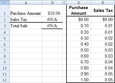
Now when we type this statement in to cell B2 our spreadsheet will look as shown above. This way the user can see that something is wrong and they should look at the input numbers to see why. The NA causes the SUM function to return NA as well.
One quick note is that there can be several ways in which you can do an IF function and they are all correct. For example when using an IF statement you can have your condition C3>40 or C3<40. The difference is that your actions would be switched around.
Cell Protection
You may want to use cell protection to keep people (including yourself) from deleting or typing over a function, formula, number or label. This is a way to customize your spreadsheet so that people can only enter into the spreadsheet the input numbers and not change any of your formulas.
Looking at the Sales tax spreadsheet Figure 8 we would not want someone to simply type over “NA”, after all that was a hard formula to develop. In fact the only place that we would want someone to type any information into would be the purchase price located in cell B1. We can accomplish this by protecting our worksheet
Cell protection is a two step process:
![]() Step
one: Format the input cells (in our example cell B1) to unlocked. This is
done through Home Tab, Cells Group, Format, Lock Cell. By default
the cell is Locked (hence the yellow color). When the cell is unlocked the
yellow is gone.
Step
one: Format the input cells (in our example cell B1) to unlocked. This is
done through Home Tab, Cells Group, Format, Lock Cell. By default
the cell is Locked (hence the yellow color). When the cell is unlocked the
yellow is gone.
Step two: Is to turn the protection
feature on. This is done through Home Tab,
Cells Group, Format, ![]() . Until you
turn this feature on, the locked/unlocked cells do not mean a thing. You can
give this protection a password so that no one can turn the feature off unless
they know the password. This option will change to
. Until you
turn this feature on, the locked/unlocked cells do not mean a thing. You can
give this protection a password so that no one can turn the feature off unless
they know the password. This option will change to ![]() when
the spreadsheet is protected. For this class you should leave the first two
check boxes checked.
when
the spreadsheet is protected. For this class you should leave the first two
check boxes checked.
You should turn the sheet protection on only after you have finished your spreadsheet. If you need to make a change to something you will need to turn the sheet protection off, make your change and then turn the protection feature back on.
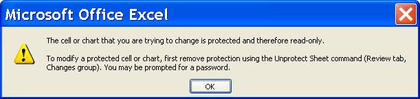
When someone tries to change a cell that is locked, a message box appears and says that you can not change a locked cell. You will also notice that a lot of the icons and options in the pull down menus have become grayed out, meaning they are not available because you have protected the document.
 A really neat feature of protecting your
spreadsheet is that you can use the tab key to move from one unprotected cell
to the next unprotected cell. Inform the person using the spreadsheet of this
by telling them to hit the tab key after they type in the information into a
cell. The cursor will then automatically go to the next input cell. One thing
to keep in mind is that this tab feature will move across the columns and then
go down to the next row. In other words if you have cells A1:B2 unlocked and
you have protected your document, when you press the tab key you will move from
A1 to B1. Then you will go to A2 then B2. Then you will go back to A1. You may
want to think about this as you are designing your spreadsheet layout. In
Figure 9 the cursor will not move from cell B1 since we have only one
unlocked cell.
A really neat feature of protecting your
spreadsheet is that you can use the tab key to move from one unprotected cell
to the next unprotected cell. Inform the person using the spreadsheet of this
by telling them to hit the tab key after they type in the information into a
cell. The cursor will then automatically go to the next input cell. One thing
to keep in mind is that this tab feature will move across the columns and then
go down to the next row. In other words if you have cells A1:B2 unlocked and
you have protected your document, when you press the tab key you will move from
A1 to B1. Then you will go to A2 then B2. Then you will go back to A1. You may
want to think about this as you are designing your spreadsheet layout. In
Figure 9 the cursor will not move from cell B1 since we have only one
unlocked cell.
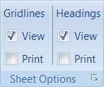
Gridlines
Once you start formatting your spreadsheet with borders, you may decide that you do not want to look at the gridlines or print them anymore. If you do not want to print the gridlines you would turn the check box off that is found under Page Layout Tab, Sheet Options Group, Print Check box. You can choose to not show the gridlines on the screen as well. In this case the gridlines will be showing on the screen but not printed.
Naming and Deleting Sheets
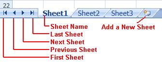 It
is real easy to name sheets. The sheet names are all at the bottom and you can
move between them by clicking on the name or using the sheet navigation buttons
shown in Figure 13. You should name your sheets with an appropriate or
relevant name. Simply have the sheet active double click on the sheet name and
then type in the name you want to give it.
It
is real easy to name sheets. The sheet names are all at the bottom and you can
move between them by clicking on the name or using the sheet navigation buttons
shown in Figure 13. You should name your sheets with an appropriate or
relevant name. Simply have the sheet active double click on the sheet name and
then type in the name you want to give it.
You
should also delete the extra sheets that you are not using. On the Home tab, Cells Group, Delete, ![]() .
.
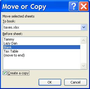
You can also copy a sheet that you have completed. On the Home tab, in the Cells group, click Format, and then under Organize Sheets, click Move or Copy Sheet. Click on the sheet that you want to copy (this is where having descriptive names comes in handy) and click on the Create a Copy check box. This will create a copy of the sheet that you have specified including all your formatting features.
Referring to cells in a different sheet
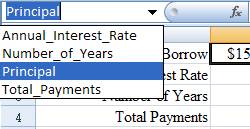 You
can refer to cells in another sheet by using the range name. Just start typing
the formula or function as you would normally. When you get to the part that
you want a range name just type that name in or choose the list box on the
formula bar as shown in Figure 21. This will present you with a list of range
names that are available in this workbook. Just choose the correct name. If you
are trying to refer to cells that are not named just use your mouse to click on
the sheet and then highlight the cell range that you want.
You
can refer to cells in another sheet by using the range name. Just start typing
the formula or function as you would normally. When you get to the part that
you want a range name just type that name in or choose the list box on the
formula bar as shown in Figure 21. This will present you with a list of range
names that are available in this workbook. Just choose the correct name. If you
are trying to refer to cells that are not named just use your mouse to click on
the sheet and then highlight the cell range that you want.
When
you refer to a cell in another sheet you will notice that Excel will put the
sheet’s name as well as the cell name in the formula. This is called the
syntax. If you wanted to type the cell reference you can as long as you include
the correct syntax in this form: ’sheetname’!cellreference. Where the
sheetname is simply the name of the  sheet,
cell reference is the cell or range of cells and they are both separated by the
! with no spaces.
sheet,
cell reference is the cell or range of cells and they are both separated by the
! with no spaces.
To continue typing in the function just type the comma, parenthesis or math operator and this will bring you back to the sheet where you have the formula that you are working on.
What’s wrong with this function
=PMT(0.899/12,48,15,000)
Two things are wrong with this function. First there are no cell references! Always use a cell reference when possible. The second thing wrong is the comma in 15,000. The computer will think that the comma is separating parameters and that your principal is 15 instead of 15,000!
Here is a list of error messages that may show up in a cell and their meanings as taken from the Microsoft Excel Help file.
Error value Meaning
#DIV/0! The formula is trying to divide by zero.
#N/A No value is available. Usually, you enter this value directly into worksheet cells that will eventually contain data that is not yet available. Formulas referring to those cells will return #N/A instead of calculating a value.
#NAME? Microsoft Excel does not recognize a name used in the formula.
#NULL! You specified an intersection of two areas that do not intersect.
#NUM! There is a problem with a number.
#REF! The formula refers to a cell that is not valid.
#VALUE! An argument or operand is of the wrong type.
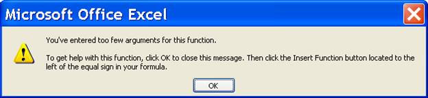
Sometimes when you forget a required parameter you will get a message that
looks like Figure 24. In this case I forgot to include the principle
amount in the PMT function. If you do not see right away what is wrong with the
function by looking at the help tip then try looking the function up to get
more detailed information.